How Distance Impacts Delivery Time and Ways to Optimize for Customer Satisfaction
Problem Statement
Quick commerce is a rapidly evolving business in India, projected to grow to $10 billion by 2029, according to a Times of India report. In this context, businesses want to understand how distance impacts delivery time and explore ways to optimize it to improve customer satisfaction.
To address this, we’ll solve the problem using SQL. Let’s start by creating a sample data table in MySQL.
Sample code for analyzing relation between distance and time
CREATE TABLE delivery (
    order_id INT,
    delivery_start_time DATETIME,
    delivery_end_time DATETIME,
    distance_covered FLOAT
);

INSERT INTO delivery (order_id, delivery_start_time, delivery_end_time, distance_covered) VALUES
(1, '2024-10-25 10:00:00', '2024-10-25 10:30:00', 5.0),
(2, '2024-10-25 11:00:00', '2024-10-25 11:45:00', 10.0),
(3, '2024-10-25 12:00:00', '2024-10-25 12:35:00', 7.0),
(4, '2024-10-25 13:00:00', '2024-10-25 13:20:00', 4.0),
(5, '2024-10-25 14:00:00', '2024-10-25 14:55:00', 12.0),
(6, '2024-10-25 15:00:00', '2024-10-25 15:25:00', 6.5),
(7, '2024-10-25 16:00:00', '2024-10-25 16:40:00', 9.0),
(8, '2024-10-25 17:00:00', '2024-10-25 17:30:00', 8.0),
(9, '2024-10-25 18:00:00', '2024-10-25 18:50:00', 11.0),
(10, '2024-10-25 19:00:00', '2024-10-25 19:35:00', 10.5);
The above delivery details represent the following table format:
| Order ID | Start Time | End Time | Distance (km) |
|---|---|---|---|
| 1 | 2024-10-25 10:00 | 2024-10-25 10:30 | 5.0 |
| 2 | 2024-10-25 11:00 | 2024-10-25 11:45 | 10.0 |
| 3 | 2024-10-25 12:00 | 2024-10-25 12:35 | 7.0 |
| 4 | 2024-10-25 13:00 | 2024-10-25 13:20 | 4.0 |
| 5 | 2024-10-25 14:00 | 2024-10-25 14:55 | 12.0 |
| 6 | 2024-10-25 15:00 | 2024-10-25 15:25 | 6.5 |
| 7 | 2024-10-25 16:00 | 2024-10-25 16:40 | 9.0 |
| 8 | 2024-10-25 17:00 | 2024-10-25 17:30 | 8.0 |
| 9 | 2024-10-25 18:00 | 2024-10-25 18:50 | 11.0 |
| 10 | 2024-10-25 19:00 | 2024-10-25 19:35 | 10.5 |
Now we have order_id, start_time, end_time, and distance. In order to analyze the relation between distance covered and delivery time, we can use correlation metrics. Let's proceed with Pearson's correlation coefficient.
\( r = \frac{\sum (X - \overline{X})(Y - \overline{Y})}{\sqrt{\sum (X - \overline{X})^2 \cdot \sum (Y - \overline{Y})^2}} \)
Where:
\( \overline{X} \): Mean Average Time
\( \overline{Y} \): Mean Average Distance
-
Pearson's correlation (PC) tells us about the linear relationship between 2 variables. In this case, the variables are distance and delivery time. PC gives values between +1 and -1:
- +1: Positive relation (as distance increases, time increases).
- 0: No relation between distance and time.
- -1: Negative relation (as distance increases, time decreases).
- Now let's find out how the Pearson Correlation Coefficient can be implemented here using SQL.
WITH cte AS (
    SELECT order_id, delivery_start_time, delivery_end_time,
    distance_covered,
    TIMESTAMPDIFF(MINUTE, delivery_start_time, delivery_end_time) AS delivery_time
    FROM delivery
)
,cte2 AS (
    SELECT ROUND(AVG(distance_covered),2) AS avg_distance,
    ROUND(AVG(TIMESTAMPDIFF(MINUTE, delivery_start_time,delivery_end_time) ),2) AS avg_delivery_time
    FROM delivery
)
, cte3 AS(
    SELECT c1.distance_covered,
    c1.delivery_time,
    c2.avg_distance,c2.avg_delivery_time,
    (c1.distance_covered - c2.avg_distance) * (c1.delivery_time - c2.avg_delivery_time) AS covariance,
    POWER((c1.distance_covered - c2.avg_distance),2) AS covariance_distance,
    POWER((c1.delivery_time - c2.avg_delivery_time),2) AS covariance_time
    FROM cte c1, cte2 c2
)
SELECT
ROUND(sum(covariance) *1.0 /
      SQRT(sum(covariance_distance) * sum(covariance_time) ),3) AS pearson_correlation
FROM cte3;
Step-by-step Execution:
-
First, from the delivery data, we calculated delivery time using
delivery_start_time&delivery_end_time.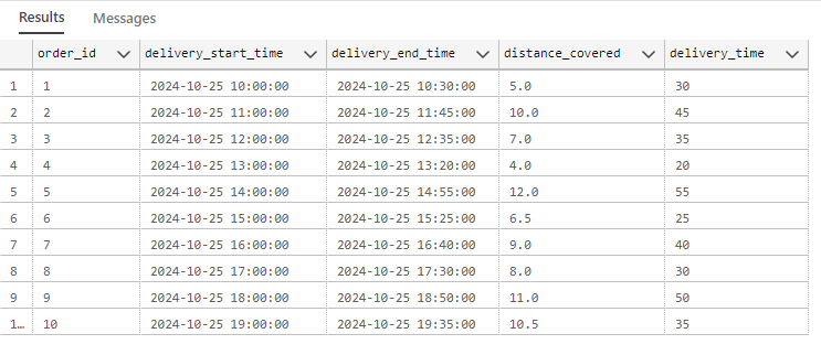
-
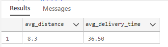
Next, to implement Pearson correlation, we need the average time and average distance, which was calculated in CTE2.
-
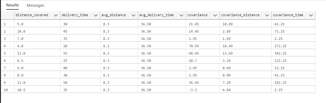
In CTE3, we calculated the covariance of distance and time to see the magnitude of the relation between them.
-
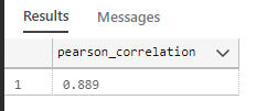
Finally, Pearson correlation is implemented in the last CTE, resulting in a value of 0.889. This indicates a strong positive correlation.
Conclusion & Business Impact
- Predictive Power: This metric is useful for future orders. If we know the distance, we can reliably estimate the delivery time.
- Operational Efficiency: By understanding this relation, we can deploy staff efficiently during peak hours, optimize routing, and strategically place dark stores.
- Data-Driven Decisions: The Pearson correlation provides a quantitative measure to support decisions around delivery efficiency and cost-effectiveness, ultimately improving customer satisfaction.